Linear Regression and PCA¶

Writing my own Linear Regression and Principle Component Analysis functions and applying them to real data sets.¶

import numpy as np 
import matplotlib.pyplot as plt 
from scipy import stats
import pandas as pd
from sklearn.decomposition import PCA
import warnings
warnings.filterwarnings('ignore')

Linear regression¶

To calculate the slope and intercept, I solved the normal equation below, where \(\beta\) is the vector of parameters (slope and intercept), \(A\) is the matrix containing a column of x values and a column of ones, \(A^T\) is its transpose, and \(y\) is the column vector of y values:

\[ (A^T A) \beta = A^T y \]

To calculate the coefficient of determination:

\[ r^2 = \frac{Cov(X,Y)^2}{Var(X)Var(Y)}\]

def lin_reg_func (exp_vec, res_vec):
    ones = np.array([1]*len(exp_vec))
    A = np.column_stack((ones,exp_vec))
    T = A.T
    a = T@A
    b = T@res_vec
    beta = np.linalg.solve(a,b)
    r2 = (np.cov(exp_vec,res_vec))**2 / (np.var(exp_vec, ddof=1)*np.var(res_vec, ddof=1)) 
    return [print('m:', beta.item(1), 'int:', beta.item(0), 'r^2:', r2.item(1))]

Applying my function to macaroni pengiun excersise data with heart rate as the explanatory and oxygen consumption as the response variable.¶

macaroni = pd.read_csv("Macaroni_Penguins_Green.csv")
macaroni.head()

	Group	ID	Heart Rate	Mass Specific VO2
0	BM	cal04	96.0	10.823194
1	BM	cal04	119.0	17.088499
2	BM	cal04	162.0	29.527144
3	BM	cal04	138.4	24.419926
4	BM	cal04	108.6	11.325901

hr = macaroni['Heart Rate']
vo2 = macaroni['Mass Specific VO2']

#my function
print('MY FUNCTION')
lin_reg_func(hr, vo2)

#double check with built in linregress function
slope, intercept, r, p_value, std_err = stats.linregress(hr,vo2)
print('BUILT IN FUNCTION')
print("m:        ", slope)
print("intercept:", intercept)
print("r^2:      ", r**2)

MY FUNCTION
m: 0.18035385335380472 int: -2.8688217734099393 r^2: 0.4908281215079641
BUILT IN FUNCTION
m:         0.18035385335380294
intercept: -2.868821773409703
r^2:       0.490828121507964

Plotting residuals of the model to check assumptions made when performing linear regression¶

def residual_func (exp_vec, res_vec):
    ones = np.array([1]*len(exp_vec))
    A = np.column_stack((ones, exp_vec))
    T = A.T
    a = T@A
    b = T@res_vec
    beta = np.linalg.solve(a,b)
    m = beta.item(1)
    intercept = beta.item(0)
    vo2_prediction = intercept + m*exp_vec
    return res_vec - vo2_prediction

residuals = residual_func(hr, vo2)
plt.scatter(hr, residuals)
plt.title('Residuals')
plt.xlabel('Heart Rate')
plt.ylabel('Residuals')
plt.axhline(y=0)
plt.show()

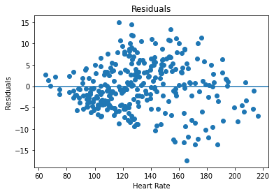
The residual plot does look consistent with the assumption of linear regression because it appears to be a random cloud of points around the horizontal axis.

PCA Function¶

Inputs: n x m matrix of data, the dimension along which to perform PCA (0 or 1 - rows or columns), and the number (k) of principal components to return.

Outputs: k principal components and their respective coefficients of determinaton

def pca_func(X, d, k):
    matrix = np.array(X)
    if d == 0:
        covmat = np.cov(matrix, rowvar = True)  
    if d == 1:
        covmat = np.cov(matrix, rowvar = False)
    eigval, eigvec = np.linalg.eig(covmat)
    eigval = np.real(eigval)
    eigvec = np.real(eigvec)
    index = eigval.argsort()[::-1]
    eigval = eigval[index]
    eigvec = eigvec[:,index]
    var = []
    for i in range(len(eigval)):
        var.append(eigval[i] / np.sum(eigval))
    return eigvec[:,0:k], var

Applying my PCA function to a gene expression dataset¶

The Spellman dataset provides the gene expression data measured in Saccharomyces cerevisiae cell cultures that have been synchronized at different points of the cell cycle. References here: http://finzi.psych.upenn.edu/library/minerva/html/Spellman.html

spellman = pd.read_csv("Spellman.csv")
spellman.head()

	time	YAL001C	YAL014C	YAL016W	YAL020C	YAL022C	YAL036C	YAL038W	YAL039C	YAL040C	...	YPR189W	YPR191W	YPR193C	YPR194C	YPR197C	YPR198W	YPR199C	YPR201W	YPR203W	YPR204W
0	40	-0.07	0.215	0.15	-0.350	-0.415	0.540	-0.625	0.05	0.335	...	0.13	-0.435	-0.005	-0.365	0.015	-0.06	0.155	-0.255	0.57	0.405
1	50	-0.23	0.090	0.15	-0.280	-0.590	0.330	-0.600	-0.24	0.050	...	0.08	-0.130	0.020	-0.590	0.100	0.08	0.190	-0.360	0.12	0.170
2	60	-0.10	0.025	0.22	-0.215	-0.580	0.215	-0.400	-0.19	-0.040	...	-0.06	-0.350	-0.180	-0.550	0.210	0.21	0.235	-0.300	-0.07	-0.045
3	70	0.03	-0.040	0.29	-0.150	-0.570	0.100	-0.200	-0.14	-0.130	...	-0.20	-0.570	-0.380	-0.510	0.320	0.34	0.280	-0.240	-0.26	-0.260
4	80	-0.04	-0.040	-0.10	0.160	-0.090	-0.270	-0.130	-1.22	0.020	...	0.05	-0.210	0.030	0.390	0.110	0.65	-0.260	1.300	-0.44	-0.600

5 rows × 4382 columns

#remove time column
spellman_genes = spellman.iloc[:,np.arange(1,4382)]

#run pca function
spell_pca = pca_func(spellman_genes, 1, 10)

#extract variance of top 10 eigenvalues
eigval_10 = spell_pca[1][0:10]
pcs = np.arange(0,10,1)

plt.plot(pcs, eigval_10)
plt.xlabel('Principal Component')
plt.ylabel('Fraction of Variance')
plt.title('Fraction of variance explained by first 10 Eigenvalues')
plt.show()

print('Total variance explained by the first 10 eigenvalues:', sum(eigval_10))

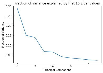
Total variance explained by the first 10 eigenvalues: 0.8611359654492433

Alice's Projects

Linear Regression and PCA¶

Writing my own Linear Regression and Principle Component Analysis functions and applying them to real data sets.¶