
Gradient Optimization
import numpy as np
import matplotlib.pyplot as plt
import pandas as pd
from scipy import stats
import warnings
warnings.filterwarnings('ignore')
Writing my own functions for different gradient optimization methods and using them to fit data.
KaiC_data.csv contains the data of concentration of the circadian protein KaiC as a function of time. The file contains two variables: Time (in hours) and KaiC (in arbitrary units)
#reading in the data
KaiC = pd.read_csv("data/KaiC_data.csv")
Time = np.array(KaiC.Time)
Amount = np.array(KaiC.Amount)
Italy_COVID.csv contains the data (case counts) from the first two months of the COVID outbreak for all of Italy
Italy = pd.read_csv("data/Italy_COVID.csv")
cases = Italy.cases
time = np.arange(0, len(cases))
Multidimensional optimization of Quadratic Functions
Quadratic function with known linear and quardatic terms:
(where f(x) is a scalar, x is a vector, b is a vector, and A is a matrix)
#values to use in the functions
A1 = np.array([[2, 1],[ 1, 2 ]])
b1 = np.array([5, -2])
#necessary functions

#quadratic function
def quad_func(A,b,x):
    return (1/2)*x.T@A@x - b@x

#gradient function
def gradient_func(A,b,x):
    return (1/2)*A.T@x + (1/2)*A@x - b.T

x = np.array([0,1])
print(quad_func(A1,b1,x))
print(gradient_func(A1,b1,x))
3.0
[-4.  4.]
Gradient Descent Function
def gradient_descent_func(A,b,x0,max_step,tol):
    step = 0
    r = 1
    diff = 100
    old_value = quad_func(A,b,x0)
    while step < max_step and diff > tol:
        new_vec = x0 - r*gradient_func(A,b,x0)
        new_value = quad_func(A,b,new_vec)
        if new_value<old_value:
            diff = np.linalg.norm(new_vec - x0)
            step = step+1
            x0 = new_vec
            old_value = new_value
        else:
            r = r/2
    return x0, step

x0 = np.array([5,15])
tol = 1*10**(-5)

print(gradient_descent_func(A1, b1, x0, 10000, tol))
print(np.linalg.solve(A1,b1))
(array([ 3.99999785, -3.00000012]), 23)
[ 4. -3.]
The given gradient descent function took 23 steps to converge to the given tolerance level.
Newton-Raphson Method
def newton_func(H,b,x0,max_step,tol):
    step = 0
    diff = 100
    old_value = quad_func(H,b,x0)
    while step < max_step and diff > tol:
        new_vec = x0 - np.linalg.inv(H)@gradient_func(H,b,x0)
        new_value = quad_func(H,b,new_vec)
        diff = np.linalg.norm(new_vec - x0)
        step = step+1
        x0 = new_vec
        old_value = new_value
    return x0, step

x0 = np.array([5,15])
tol = 1*10**(-5)

print(newton_func(A1, b1, x0, 10000, tol))
print(np.linalg.solve(A1,b1))
(array([ 4., -3.]), 2)
[ 4. -3.]
Using the Newton-Raphson method, the function converged much faster taking only two steps.
Levenberg-Marquardt Method
def lm_func14(H,b,x0,max_step,tol):
    step = 0
    diff = 100
    old_value = quad_func(H,b,x0)
    lamda = 100.0
    s = 5
    while step < max_step and diff > tol:
        new_vec = x0 - np.linalg.inv(H + lamda*np.diag(np.diag(H)))@gradient_func(H,b,x0)
        new_value = quad_func(H,b,new_vec)
        if new_value < old_value:
            diff = np.linalg.norm(new_vec - x0)
            step = step+1
            x0 = new_vec
            old_value = new_value
            lamda = lamda/s
        else:
            lamda = lamda*s
    return x0, step

x0 = np.array([5,15])
tol = 1*10**(-5)

print(lm_func14(A1, b1, x0, 10000, tol))
print(np.linalg.solve(A1,b1))
(array([ 4., -3.]), 9)
[ 4. -3.]
Using the Levenberg-Marquardt method, the function took 9 steps to converge.
Nonlinear Least Squares Optimization
Using the Levenberg-Marquardt method to perform a nonlinear least squares fit, using the exponential decay function with parameters \(a\) and \(k\):
Auxilliary functions
Function to compute the sum of square errors (the objective function)
\[ SSE = \sum_i (ae^{kx_i} - y_i)^2 \]Function to calculate the gradient (G) and Hessian (H) for the nonlinear least squares optimization
The gradient component in the direction of parameter a is the sum over all data points of the following term: $\( G[0] = \sum_i (f(x_i; a, k)-y_i) \frac{\partial f(x_i; a, k)}{\partial a}\)$
The gradient component in the direction of parameter k is the sum over all data points of the following term: $\( G[1] = \sum_i (f(x_i; a, k)-y_i) \frac{\partial f(x_i; a, k)}{\partial k}\)\( Here \)y_i = f(x_i; a, k)$, and SSE is calculated by the first function.
The Hessian matrix is then computed as follows: $\(H[0,0] = \sum_i \left(\frac{\partial f (x_i; a, k)}{\partial a} \right)^2 \)\( \)\(H[1,1] = \sum_i \left(\frac{\partial f (x_i; a, k)}{\partial k}\right)^2\)\( \)\(H[0,1] = H[1,0]= \sum_i \frac{\partial f (x_i; a, k)}{\partial a} \frac{\partial f (x_i; a, k)}{\partial k}\)$
Test my functions with KaiC data, using parameters a=10 and k=-0.5. I should get:
SSE = 3397.7197634698623 G = [[ -72.80278399],[-348.94647508]] H = [[1.58196699, 9.20551297],[9.20551297, 199.07470824]]
def se_func (x,a,k):
    return a*np.exp(k*x)
def sse_func (x,y,a,k):
    return np.sum((se_func(x,a,k) - y)**2)

a = 10
k = -0.5
sse_func(KaiC.iloc[:,0], KaiC.iloc[:,1],a,k)
3397.7197634698623
def grad_hess_func (x,y,a,k):
    G = np.zeros(2)
    H = np.array([[0.0, 0.0],[ 0.0, 0.0]])
    se = a*np.exp(k*x) - y
    pa = np.exp(k*x)
    pk = a*x*np.exp(k*x)
    G[0] = np.sum(se * pa)
    G[1] = np.sum(se * pk)
    H[0,0] = np.sum(pa**2)
    H[1,1] = np.sum(pk**2)
    H[1,0] = np.sum(pa*pk)
    H[0,1] = H[1,0]
    return G, H

a = 10
k = -0.5
grad_hess_func(KaiC.iloc[:,0], KaiC.iloc[:,1],a,k)
(array([ -72.80278399, -348.94647508]),
 array([[  1.58196699,   9.20551297],
        [  9.20551297, 199.07470824]]))
Modifying my function to implement the Levenberg-Marquardt method for finding best-fit parameters a and k for exponential curve-fitting
def lm_func22(a0,k0,x,y,max_step,tol,scale):
    step = 0
    diff = 100
    old_vec = np.array([a0, k0])
    old_value = sse_func(x,y,a0,k0)
    lamda = 100.0
    while step < max_step and diff > tol:
        G,H = grad_hess_func(x,y,a0,k0)
        new_vec = old_vec - np.linalg.inv(H + lamda*np.diag(np.diag(H)))@G
        a0, k0 = new_vec
        new_value = sse_func(x,y,a0,k0)
        if new_value < old_value:
            diff = np.linalg.norm(new_vec - old_vec)
            step = step+1
            old_vec = new_vec
            old_value = new_value
            lamda = lamda/scale
        else:
            lamda = lamda*scale
    a0, k0 = old_vec
    return a0, k0, step
a0 = 10
k0 = -0.5
tol = 1*10**(-5)

Kai_lm = lm_func22(a0,k0,KaiC.iloc[:,0], KaiC.iloc[:,1],1000,tol,3)
Kai_lm
(59.28974011690078, -0.605985748917563, 13)
amount_kai = se_func(Time, Kai_lm[0], Kai_lm[1])
plt.scatter(Time, Amount, label = 'data')
plt.plot(Time, amount_kai, 'orange', label = 'LM fit')
plt.title('KaiC amount over Time')
plt.xlabel('Time (hrs)')
plt.ylabel('KaiC amount')
plt.legend()
plt.show()

SSE_kai = sum((amount_kai - Amount)**2)
print('SSE:', SSE_kai)
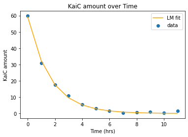
SSE: 7.243426946877536
The SSE is fairly low, and the fit looks good.
Fitting Covid data from Italy
a0 = 0.5
k0 = 0.05
tol = 1*10**(-2.5)
time = time.astype(float)
cases = cases.astype(float)
covid_lm = lm_func22(a0,k0,time,cases,1000,tol,8)
covid_lm
(251.71073271305258, 0.10639127757098622, 70)
cases_covid = se_func(time, covid_lm[0], covid_lm[1])

plt.scatter(time, cases, label = 'data')
plt.plot(time, cases_covid, 'orange', label = 'LM fit')
plt.title('New Cases over Time')
plt.xlabel('Time (days)')
plt.ylabel('New Cases')
plt.legend()
plt.show()

SSE_covid = sum((cases_covid - cases)**2)
print('SSE:', SSE_covid)
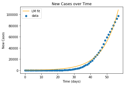
SSE: 699403404.0976192
There is a higher SSE and the fit appears a bit too steep compared to the actual data.